Setting up and Running Gaussian Jobs

This chapter discusses setting up and running Gaussian calculations with GaussView. It deals only with the mechanics of doing so. Consult the Gaussian 09 User’s Reference for detailed information about all Gaussian 09 keywords and options.

The Gaussian Calculation Setup Window

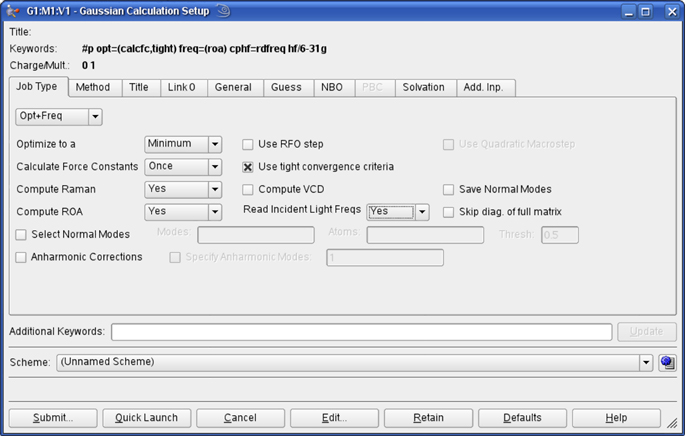
The first step in producing a Gaussian input file is to build the desired molecule. The bond lengths, bond angles, and dihedral angles for the molecule will be used by GaussView to write a molecular structure for the calculation. Once this is completed, you can use the Calculate=>Gaussian Calculation Setup menu path to open the Gaussian Calculation Setup dialog. It is illustrated in Figure 67.

Figure 67. The Gaussian Calculation Setup Dialog

This dialog allows you to set up virtually all types of Gaussian calculations and to submit them from GaussView. The route section that GaussView is generating appears at the top of the dialog, and it is constantly updated as you make selections in the dialog.

The Gaussian Calculation Setup dialog contains several panels, described individually below. The buttons at the bottom of the dialog have the following effects:

• Submit: Starts a Gaussian calculation using the current input file. You will be prompted to save the input file if you have not already done so.
• Quick Launch: Launches a Gaussian job without further ado (discussed later in this section).
• Cancel: Closes the dialog box and returns all selections to their default values.
• Edit: Allows direct access to the input file with an external text editor. The input file is not available for editing until it has been saved with GaussView.
• Retain: Closes the dialog box. Current selections are retained, but the input file is not created/updated, and no Gaussian job is submitted.
• Defaults: Returns all items to their default values.
• Help: Provides online help for this dialog.

The Job Type Panel

The Job Type panel appears in Figures 67 and 68. The top popup menu selects the job type. The default is a single point energy calculation. The remaining fields in the panel represent common options for the selected job type (Figure 67 shows the ones for an Opt+Freq calculation).

In order to select a different job type than those listed in the popup menu, select the blank menu item at the bottom of the list, and then type the appropriate Gaussian keyword into the Additional Keywords section in the lower section of the dialog.

You can also use this field to add any desired Gaussian keyword and/or option. In the latter case, you must repeat the keyword within this field even if it already appears in the route section. GaussView will merge all options for the same keyword within the route section (see Figure 68 for an example). Note that this area is designed only for adding keywords to the route section. Use the Edit button for creating complex input files.

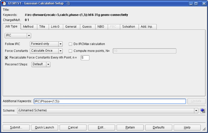
Figure 68. Adding an Option via the Additional Keywords Field

This window illustrates GaussView’s ability to merge options selected from dialog controls with ones typed into the Additional Keywords field. Here, we’ve added the Phase option to the IRC keyword, while another option has been generated with the Calculate Force Constants popup selection.

The Scheme field at the bottom of the dialog is used to quickly retrieve a stored set of keywords and options. This feature is described later in this chapter.

The Method Panel

The Method panel specifies the quantum mechanical method to be used in a calculation. The default method is a ground state, closed shell Hartree-Fock calculation using the 3-21G basis set. This panel is illustrated in Figure 69.

The fields in the Method line specify the following items:

• Whether the calculation is for a ground state or an excited state.
• The theoretical method. For some choices, a fourth field is used to select the specific method of the given type. For example, in Figure 69, the method field is set to DFT, and the fourth field selects the B3LYP functional.
• The wavefunction type (closed shell vs. open shell). The default is an unspecified type. The Restricted, Unrestricted, and Restricted-Open selections prepend R, U and RO to the method keyword (respectively).

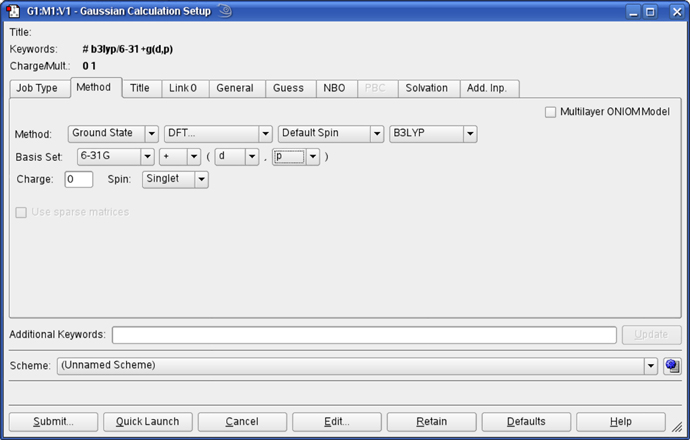
Figure 69. The Method Panel

The Method panel is where the model chemistry for the calculation is specified.

The Basis Set menus allow the selection of the basis set to be used in the calculation. Polarization functions and diffuse functions may be added to the basis set using the corresponding menus in this line. Select the Custom item at the bottom of the basis set menu to select a basis set other than those that can be constructed via the controls in this area. You may enter any basis set keyword in the name field:

Figure 70. Entering a Custom Basis Set Keyword

The Charge and Spin fields specify the molecule’s charge and spin multiplicity. GaussView will select values for these fields based on the molecular structure. They may be modified as needed.

The Title Panel

The Title panel holds a field used for the Gaussian title section (designed to contain a brief description of the job). Type your description into the text box.

The Link 0 Panel

The Link 0 panel is used for entering Link 0 commands for the job (see Figure 71). Note that if you remove the specification for the name and location of the checkpoint file, you will not be able to visualize output automatically from this job.

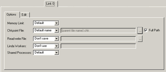
Figure 71. The Link 0 Panel

This panel specifies a name for the checkpoint file and the read-write file, the amount of memory to use for this job, the number of shared memory processors and/or the locations of Linda workers. You can specify the various settings via controls in the Options subpanel. Alternatively, you can edit the Link 0 commands directly using the Edit subpanel. The Full Path checkbox controls whether an absolute path (checked) is used with %Chk/

The General Panel

The General panel allows you to select commonly used general calculation options. It is illustrated in Figure 72.

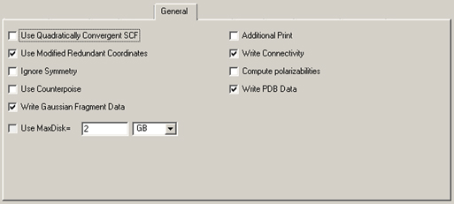
Figure 72. Selecting General Gaussian Options

This panel contains a set of commonly used options. This window illustrates the defaults.

The following table indicates the Gaussian keywords corresponding to these items:

The Use Modified Redundant Coordinates item is enabled only if you have set up redundant coordinates with the Redundant Coordinate Editor. If not, the item is ignored (despite its default value). Write Gaussian Fragment Data and Write PDB Data are enabled by default, but have no effect unless the corresponding items are defined.

The Write Connectivity option also includes the appropriate additional input section(s) in the Gaussian input file.

Note: Consult the discussion of the SCF keyword in the Gaussian 09 User’s Reference for recommendations for unusual/problem cases (SCF=QC is not always the best next choice).

The Guess Panel

Th Guess panel contains settings related to the initial guess. It is illustrated in Figure 73. Consult the discussion of the Guess keyword in the Gaussian 09 User’s Reference for full details on these options.

The Guess Method popup specifies the type of initial guess to use. It has the following options:

• Default: Uses the default Harris initial guess.
• Core Hamiltonian: Uses the Gaussian 98 default initial guess (Guess=INDO). Generally, we do not recomment its use except when recommended by Gaussian, Inc. technical support staff.
• Extended Huckel: Uses the Huckel guess (Guess=Huckel).
• Read checkpoint file: Retrieves the initial guess from the checkpoint file (Guess=Read).
• Read checkpoint; otherwise generate: Check checkpoint file for the initial guess; generate if not present (Guess=TCheck).
• Read input checkpoint file: Read the guess from the checkpoint file whose name is specified in the input stream (Guess=Input).

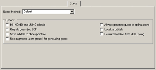
Figure 73. Gaussian Initial Guess Options

This window shows the default settings for the initial guess.

The options in this panel have the following meanings:

The Permuted orbitals for MOs Dialog is disabled unless you have specified an alternate orbital ordering with the MO Editor. If enabled, it is on by default.

The Use fragments (atom groups) for generating guess is disabled unless fragments have been defined using the Atom Group Editor. If enabled, it is checked by default. In addition, fragment-specific charges and spin multiplicities are generated and placed into the route section. You can also modify them using the Atom Group Editor (see the example for antiferromagnetic coupling in a later section of this manual).

The NBO Panel

The NBO panel is used to select NBO analysis at the conclusion of the Gaussian job. It is illustrated in Figure 74. The Type menu specifies the kind of NBO analysis to perform. The Checkpoint Save field allows you to save NBOs and/or NLMOs in the checkpoint file for later visualization (the default is Don’t Save).

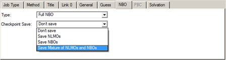
Figure 74. The NBO Panel

The panel specifies the type of NBO analysis and which NBOs to save in the checkpoint file. The selection in this window is often a useful one when you will use them to generate an active space for a CASSCF calculation.

The Solvation Panel

The Solvation panel allows you to specify that the calculation is to be performed in solution rather than in the gas phase. It is illustrated in Figure 75. The Model field allows you to specify a specific solvation model (the default is PCM, which itself defaults to IEFPCM). You can also specify the solvent by selecting it from the corresponding popup menu. Use the Other selection to select a solvent other than those on the list; you will need to specify within the route section manually (e.g., placing SCRF(EPS=value) within the Additional Keywords field).

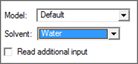
Figure 75. The Solvation Panel

This panel specifies the SCRF model to use for solvent effects. The Default selection corresponds to the Gaussian default of SCRF=PCM.

Note that some solvation models may present different/additional fields for their required parameters. You may use the Read additional input box to generate the SCRF=Read option; additional input may be entered using the Add. Inp. panel (see below).

The PBC Panel

The PBC panel is used to specify options to the Gaussian PBC keyword (see Figure 68). Checking the Use PBC box causes the translation vectors to be added to the molecule specification. This is the default when a unit cell has been defined with the Crystal Editor. The panel is disabled for non-periodic systems.

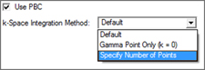
Figure 76. The PBC Panel

The Use PBC checkbox causes the translation vectors to be placed in the molecule specification. After you select the option above, an additional field for specifying the number of K-points will appear.

The Additional Input Panel

The final panel in the Gaussian Calculation Setup dialog is labeled Add. Inp. It may be used to enter any additional input section(s) required by the calculation you plan to run. This input will be written to the Gaussian input file provided that Append Extra Input is checked in the Save dialog. Any additional input present in input files that you open will also appear in this panel.

Special Considerations for Various Gaussian Job Types

This section summarizes information about setting up various Gaussian job types for which some special steps are required. All GaussView features mentioned are discussed in detail earlier in this book.

Transition Structure Optimizations: Opt=QST2 and Opt=QST3

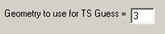
Gaussian STQN-based transition structure optimizations require two or three structures as input. To set up these jobs, you must create a molecule group containing the required number of structures. If you plan on running an Opt=QST3 job, then the transition structure initial guess is assumed to be molecule 3 unless you specify a different structure on the Job Type panel.

Once you have done so, the TS (QST2) and TS (QST3) options will be enabled in the Optimize to a field for the Optimization job type in the Job panel of the Gaussian Calculation Setup dialog.

Verifying and Specifying Atom Equivalences

In most cases, GaussView will automatically identify the corresponding atoms in the multiple structures for these transition state optimizations. However, you can verify this using the Connection Editor, accessed via the Connection Editor button on the toolbar or the Edit=>Connection Editor menu item.

Calculations on Polymers, Surfaces and Crystals

You can set up jobs for Gaussian’s Periodic Boundary Conditions facility using the Crystal Editor (reached via the Crystal Editor button or the Edit=>PBC menu path). Once you have defined a unit cell, GaussView automatically sets up PBC jobs for this structure by including the translation vectors within the molecule specification. This is indicated by the enabling of the PBC panel in the Gaussian Calculation Setup dialog, and the checked Use PBC item. Note that for normal cases, you do not need to access this panel at all and can proceed directly to setting up Gaussian input in the normal manner.

Multi-Layer ONIOM Calculations

GaussView contains several features for setting up ONIOM calculations.

Assigning Atoms to Layers

The Layer Editor allows you to graphically assign atoms to various ONIOM layers. It is accessed via the toolbar’s Select Layer button or via the Edit=>Select Layer menu item.

Assigning Molecular Mechanics Atoms Types

GaussView will assign Molecular Mechanics atoms types for UFF, Dreiding and Amber (including Amber charges) to all atoms in the molecule automatically. You can view and modify these using the Atom List Editor (reached via the Atom List Editor button on the toolbar or the Edit=>Atom List menu path).

Defining Link Atoms

GaussView will automatically assign minimal link atom information for the appropriate atoms in an ONIOM calculation. However, all link atoms are always handled in the same way, and they may require modification for your purposes. Link atoms generated by GaussView are always hydrogens (using the H_ UFF and Dreiding atom types and the HR Amber atom type, where R is the element of the linked-to atom). The only other link atom parameter which is included is the linked-to atom (the atom in the higher layer to which the current atom is bonded); all other parameters are left blank.

The Atom List Editor is often a convenient way to examine and modify link atoms for ONIOM calculations. You can use the ONIOM Layers button to view and modify link atoms easily.

Specifying the Model Chemistry for Each Layer

Once you have prepared the structure and specified all necessary parameters, you can set up an ONIOM calculation via the Method panel of the Gaussian Calculation Setup dialog. The Multilayer ONIOM Model checkbox indicates that this will be an ONIOM calculation (see Figure 77).

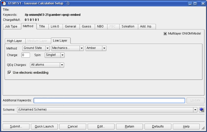
Figure 77. Setting Up a Gaussian Input File for an ONIOM Job

This example is preparing an input file for a two-layer ONIOM calculation. When Multilayer ONIOM Model is checked, the additional tabs appear in the Method panel. Each of them allows you to specify the theoretical method and basis set for the corresponding layer. In this case, we are using the Amber Molecular Mechanics method for the Low layer. Note that electronic embedding is requested by checking the final item in the Low Layer panel.

Specifying CASSCF Active Spaces Using Guess=Permute

GaussView can make it easy to specify CASSCF active space. The MOs dialog allows you to generate, view, select and reorder the starting orbitals. It is reached with the Edit=>MO Editor menu path and via the MO Editor button on the toolbar. See the detailed discussion of this tool earlier in this manual.

Modifying Redundant Internal Coordinates (Geom=ModRedundant)

You can specify additions and other modifications to redundant internal coordinates for geometry optimizations and other jobs by using the Redundant Coordinate Editor, reached via the Redundant Coordinate Editor button on the toolbar or the Edit=>Redundant Coordinates menu path. See the detailed discussion of this tool earlier in this manual.

Freezing Atoms During Geometry Optimizations

The Atom Group Editor can be used to specify atoms whose positions are to be held fixed during a geometry optimization via its Freeze Atoms group class. This class is defined with four groups by default, corresponding to unfrozen atoms, frozen atoms, and the first two ONIOM frozen rigid blocks (freeze settings of -2 and -3; see the discussion of the Geom keyword in the Gaussian 09 User’s Reference for full details on specifying frozen atoms and rigid blocks for ONIOM calculations). In order to hold specific atoms fixed during a geometry optimizations, add them to the Freeze (Yes) group in the Atom Group Editor.

Selecting Normal Modes for Frequency Calculations (Freq=SelectNormalModes)

You can use the Atom Group Editor to select atoms for which normal mode analysis is conducted (see the Gaussian 09 User’s Reference for details). Placing the desired atoms into the Select Normal Modes (Yes) group will cause them to be entered into the Atoms field corresponding to Select Normal Modes in the Gaussian Calculation Setup’s Job Type panel for Frequency jobs. You can modify this list as needed, but doing so will have no effect on the definition of the groups in the Atom Group Editor’s Select Normal Modes group class.

Calculating NMR Spin-Spin Coupling (NMR=(SpinSpin,ReadAtoms))

When you select an NMR calculation in the Gaussian Calculation Setup’s Job Type panel, the field to the left appears. The atom list in the parentheses corresponds to the members of the NMR Spin-Spin (Yes) group, as defined in the Atom Group Editor (by default, all atoms are placed into this group and the list of atoms reads all atoms). A specific group of atoms appears in this item when the NMR Spin-Spin (No) group contains at least one atom.

Specifying Fragment-Specific Charges and Spin Multiplicities

You can specify individual charge and spin multiplicity values for each fragment defined via the Atom Group Editor. This facility is useful for setting up fragment guess jobs (Guess=Fragment) for modeling antiferromagnetic coupling, counterpoise calculations (Counterpoise) for computing counterpoise corrections and basis set superposition errors, and the like. Figure 78 illustrates setting up a system for modeling antiferromagnetic coupling effects.

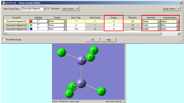
Figure 78. Specifying Per-Fragment Charge and Spin

Antiferromagnetic coupling is an effect that is important for molecules with high spin multiplicity. This Fe2Cl6 compound is a simple example. Here, we have defined three fragments. Each iron atom is in its own fragment, and the six chlorine atoms are in a third fragment. The two iron fragments are each assigned a charge of +3, and both are defined as sextets with opposite spin (i.e., spin multiplicities of 6 and -6). The fragment containing the chlorine atoms is defined as a singlet with a -6 charge. These values will be placed into the route section of the Gaussian job set up in GaussView.

The Gaussian Calculation Setup’s General panel contains features relevant to these two calculation types: Write Gaussian Fragment Data (for both types) and Use Counterpoise (for Counterpoise calculations). In addition, the Guess panel has two items useful for the first job step of a fragment guess job: Only do Guess (no SCF) and Use fragments (atom groups) for generating guess, corresponding to Guess=Only and Guess=Fragment (respectively). Typically, such a job would be followed by a second job to compute the energy including the antiferromagnetic coupling: Guess=Read Geom=AllCheck Stable=Opt.

Setting Defaults for Gaussian Jobs

The Gaussian Setup Preferences may be used to specify defaults for the Gaussian Calculation Setup dialog. Click the Calculation button, and then specify the desired settings for future Gaussian calculations. These will be applied to future job setup operations.

Defining Calculation Schemes

Modifying the Gaussian Setup Preferences as described in the preceding paragraph has the effect of modifying the Gaussian calculation scheme named Default. Schemes are named sets of calculation keywords and options, and you can define and save as many different ones as you want to. You can view the calculation scheme in effect at the bottom of the Gaussian Calculation Setup dialog and in the scheme popup in the toolbar, and in the Calculate=>Gaussian Calculation Scheme submenu. You can apply a scheme to the current molecule using any of these controls as well.

For new molecules, the Default scheme is initially applied. When you open a new molecule from a file, the scheme will be set to the scheme that matches its settings (if any) or to Unnamed Scheme.

You can view and modify the properties of the various defined schemes using the Schemes button or by selecting More Schemes from any scheme list. The resulting dialog appears in Figure 79.

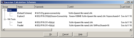
Figure 79. Viewing and Modifying Calculation Schemes

This dialog shows four schemes organized into two groups.

Any field within a scheme can be edited by clicking on it. Right clicking on a scheme produces a context menu, allowing you to add groups and schemes, cut and paste between fields, and delete schemes. You can also save schemes to an external file and load ones saved in this way back into GaussView. Note that neither the Default scheme nor the Main group may be renamed or deleted.

The Quick Launch Feature

The conventional way to run a Gaussian job from GaussView is to open the Gaussian Calculation Setup, set the correct job options, click the Submit button, and specify the name and location for the input file. The Quick Launch feature greatly simplifies this common task. A job can be launched using the Quick Launch toolbar button, the Quick Launch button in the Gaussian Calculation Setup dialog or the Calculate=>Gaussian Quick Launch menu path.

Clicking on the button in the Gaussian Calculation Setup dialog or on the portion of the toolbar icon to the left of the small arrow will immediately launch a Gaussian job using the current calculation scheme and temporary files. The toolbar icon arrow and the Calculate menu item both lead to a submenu. Its Temp File item will also result in a job started from a temporary input file. The Save File option will prompt you to save an input file and submit that file as a Gaussian job afterwards. Finally, the Save and Edit File option will prompt you to save an input file and then open that file in the external editor.

When you start a new calculation using Quick Launch a new View window is opened corresponding to it. While the job is running, a text message identifying the job, a stop button, and a stream output file button are placed in the status bar of the View window. Once the job finishes successfully, the results file is opened automatically in the same View window. When more than one results file is produced by a calculation—e.g., both a log file and a checkpoint file are created—then you will be prompted to select the file to open.

You can save the files generated from a Quick Launch operation to temporary files using the File=>Save Temp Files menu item. This item replaces the usual Related Files option under these circumstances.

Viewing and Controlling Gaussian Jobs

The Calculate=>Current Jobs menu path opens the Job Manager dialog (shown in Figure 80); the Job Manager button on the toolbar performs the same function.

This window displays all the jobs started by GaussView that are currently running. Note that only jobs started during the current session of GaussView can be displayed. Examples of jobs that may be displayed are Gaussian jobs submitted from the Gaussian dialog box, Gaussian input file edit sessions launched from GaussView, CubeGen processes for building surfaces for display, FreqChk processes to generate vibrational analysis data, and/or processes from other Gaussian utilities.

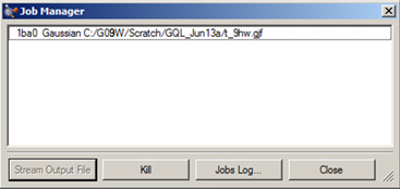
Figure 80. The Job Manager Dialog

This dialog allows you to view and control Gaussian jobs as well as jobs running Gaussian utilities like CubeGen. You can terminate a job using the Kill button.

Clicking on the Jobs Log button displays the current GaussView job log containing system messages associated with the execution of GaussView external processes. The Clear button in the resulting window removes old jobs from the job list, and the Close button dismisses the job list window.

Note that the Jobs Log button does not display the log file associated with a running Gaussian job. The latter is accomplished by the Stream Output File button for Gaussian calculations. Note that selecting this button for job types (e.g., cube generation jobs) will display whatever file GaussView can find that is associated with the job (often the Gaussian input file).

Individual jobs may be aborted using the Kill button.

Specifying How the Gaussian Program is Executed

The Job Setup Preferences dialog allows you to examine and customize how Gaussian and its utilities are launched from within GaussView. It is illustrated in Figure 81. The Application field at the top of the panel specifies the program or utility whose execution method is currently displayed. Below this popup, there are three launch choices, and the command line associated with the selected launch method is displayed in the Command Line area (where it can also be modified).

For each job type, there are three launch choices:

• Execute directly using default command line: The job will be started using the command line specified in the lower area.
• Execute indirectly through script using default command line: The job will be started using a GaussView-provided script. These scripts are located in the bin subdirectory of the GaussView installation directory. Their names are listed below. The associated command line appears in the lower area of the dialog.
• Execute using custom command line: Use the command line specified in the box to start the job. You can enter whatever command line is appropriate for your situation. The GaussView provided scripts may be called if desired.

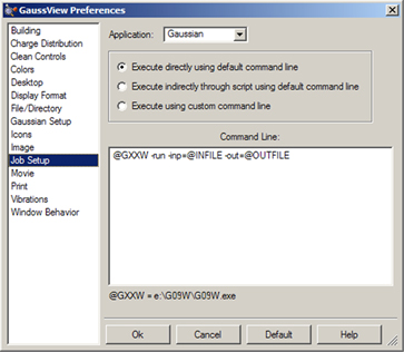
Figure 81. Job Setup Preferences

These settings are used to specify how various external jobs get initiated by GaussView.

The following figure illustrates the command line and other information displayed for running the Gaussian program using the second launch choice:

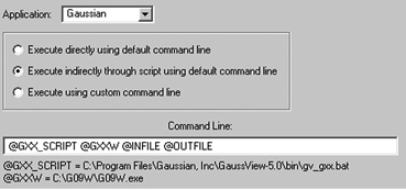
Figure 82. Running Gaussian via a Script

The Command Line field displays the command which will be used to run Gaussian via an external script (field’s height is greatly reduced). The values of the GaussView internal variables used in the command line are displayed below the field for your convenience.

GaussView provides the following scripts in its bin subdirectory:

Each script’s usage is documented in comments at the beginning of the file. Prudence dictates making a backup copy of any script before modifying it in any way. Note that all standard UNIX scripts are also provided on Mac OS X systems for your convenience.

You can specify a custom command line for external jobs using the third choice in the Job Setup Preferences dialog. However, successfully using this feature depends on a clear understanding of the command line invocation of Gaussian and its utilities under the current operating system. Consult the Gaussian 09 User’s Reference for details.

The following GaussView internal variables can be used within commands. Note that they are not operating system environment variables, despite their resemblance to them in naming conventions.